Of Loadlines, Power Output and Distortion - Part 5 - The Pentode
Purpose
In the preceding parts of this series, we concentrated on loadlines and triode operation. In this article we will explore establishing a loadline on a pentode vacuum tube (valve), determine the power available from this loadline, and the distortion predicted from this loadline. This will allow the reader a step by step way to calculate the parameters for his design. I have again chosen to "invent" a tube for illustrative purposes. My pentode has the following parameters:
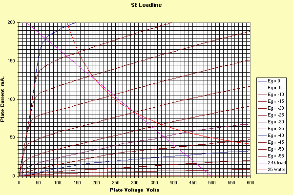
Establishing a Load Line: (very similar to a triode for S.E. applications)
For our example, the data is as follows:
Va= 70V, Vq=300V, Ve=433V, Ia=180mA, Ib=130mA, Ic=83mA, Id=51.5mA, Ie=28mA. In addition, 40V p-p are required from the driver stage, and a 2.4k plate transformer is required.
Rectification Effects
In any device with even order distortion (not just second harmonic as sometimes stated), the average current of a Class A stage will change depending on the signal level. If the distortion is relatively low, the effect is relatively unimportant, if the distortion is high, this effect becomes increasingly important. (It is also more important for self bias than fixed bias, as the bias voltage is a function of the average current).
This effect modifies all tube operating characteristics. The degree can be seen by comparing the quiescent current (83 mA in our example) with the average current as taken from the "extremes": that is, (Ia+Ie)/2. In our example that value calculates to 104mA (note that since this is reasonably different, we can expect relatively high distortion). The effect requires an iterative plot of the load line on the tube characteristics as described in part 1 of this series. Note the quiescent dissipation is still 300*0.083, or in this case 24.9 watts. The non-linearity shown here is getting dangerously close to what can be ignored, but, as we will see, the distortion in this example is too high anyway.
Power Output
Po = (Ve-Va)*(Ve-Va)/(8*loadimpedance).
In our example this is (433-70)*(433-70)/(8*2500)= 6.9 watts. This number is an approximation in that it assumes low distortion.
Second Harmonic Distortion
HD2(%) = 75*(Ia + Ie - 2*Ic)/(Ia + Ib - Id - Ie)
In our example this is 14% (!)
Third Harmonic Distortion
HD3(%) = 50*(Ia - (2*Ib) + (2*Id) - Ie)/(Ia + Ib - Id - Ie)
In our example this is -1.1%
Notice the minus sign. This indicates that the harmonic content subtracts from the fundamental (flattening it) when the fundamental is at its crest. This *usually* happens on third harmonic distortion in tubes.
Fourth Harmonic Distortion
HD4(%) = 25*(Ia - (4*Ib) + (6*Ic) - (4*Id) + Ie)/(Ia + Ib - Id - Ie)
In our example this is -2.2%
It is also possible to get an indication of how distortion varies with power output. In the example we just used, we picked 0, -10, -20, -30 and -40 volt bias points. We could also use -10, -15, -20, -25 and -30 points to see what happens at lower levels.
Applying the same formula to these points gives us 187 and 376 volts, and 130, 110.5, 83, 69.5 and 51.5 mA. This, in turn, calculates to 1.9 watts and 9.7% second harmonic, -1.5% third harmonic, and -8.5% fourth harmonic. This means the 2 watt level with this tube will also be pretty distorted!
Push Pull Operation (composite loadlines for pentodes)
We will discuss how to create a composite load line for a pentode. This is "necessary" to establish the load line for a push pull amplifier, regardless of whether it is going to be Class A or Class AB. We will continue to use the same "invented" pentode. As we will discover, establishing a realistic loadline for a pentode is slightly different than for a triode, due to the shape of the characteristic curves.
Building a Composite Load Line
This is again an iterative process, perhaps moreso than the single ended case as it's a bit more involved. Here's a step by step procedure to create a set of "composite curves" and load line.
1. Establish your intended operating point from the single ended curves. First let's consider an obvious Class A case, by choosing the same bias point we used for the single ended case: 300 volts and 83 mA quiescent current (-20 volt bias). Note: For Class AB, you may choose a lower idling current point, which will allow a lower impedance loadline (and higher power output) without exceeding maximum allowable power dissipation. For instance, choosing a -25 or -30 volt quiescent point would allow you more "room" to increase tube current. To stay within Class A operation, at least some current must flow in each tube at all bias points, otherwise, you will be operating in Class AB. In this article we will consider -20 volt bias point (requiring a swing on each of the grids of 0 to -40 volts, -25 volts (which is still technically class A, since there is some current still flowing at -50 volts bias) and -30 volts, which is Class AB, since no current flows at -60 volts bias. This is actually an important distinction with pentodes. Since the "cutoff" characteristics tend to be sloppier than a triode, most so-called Class AB amplifiers are really Class A, as some small current is flowing even at the most negative point. As we will see, truly Class AB has some pretty bad crossover (notch) distortion.
2. Since the plate voltage increases on one plate and decreases on the other plate, we must have a way of representing this. The usual method is to take another set of the same tube curves, turn them around (so the maximum current is "down" and highest plate voltage is to the "left", and position them so that the quiescent voltages line up vertically, and the zero plate current lines touch each other as shown below. I've shown the steps to do this on the curves below: that is, copy the curves, turn one around, then merge the curves as:
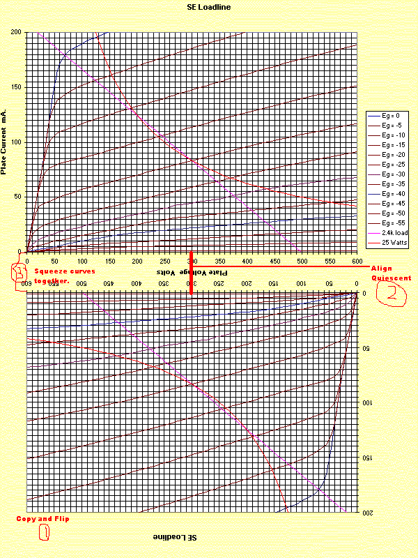
3. Now, for the chosen bias point, create a new line (labeled "composite" curve) as follows (we are going to look at ONLY the -20 volt bias lines, one on the "upper" part of the graph, one on the "lower" part of the graph:
4. You have now established one "line" of the composite curves. This is the line of varying the plate voltage symmetrically about the quiescent point while maintaining a constant grid voltage. (classic plate resistance line).
5. Now consider another set of lines for your graph. This will be the -25 volt line for the "upper" set and the -15 volt line from the lower set. (We have put a 5 volt signal into the push pull stage). Again, for each plate voltage, subtract the two currents (for instance, 310V -25V bias upper and 290 volt -15V lower) and plot the dot. Continue until you have the -25/-15V line filled in. Note that if your quiescent grid voltage was, for instance, -30 volts, the second line you would add would use the -35/-25V lines instead of -25/-15V line.
6. Next do the same for the -30/-10, the -35/-5 and -40/0 volt lines. Then do the same for the -15/-25, the -10/-30, the -5/-35 and the 0/-40 volt lines. This completes the composite curves. The last 4 curves should be mirror images of the previous 4 you filled in. Noticing this saves you some time.
7. The last thing to do is fill in the maximum power dissipation curve. There are now going to be 2 of them, one for the one tube, one for the other. These will be symmetrical about the quiescent point. It is usually necessary to graph only half of the curve. The following is for the "upper" tube. Here's how to do it:
You should now have a graph that looks like this...
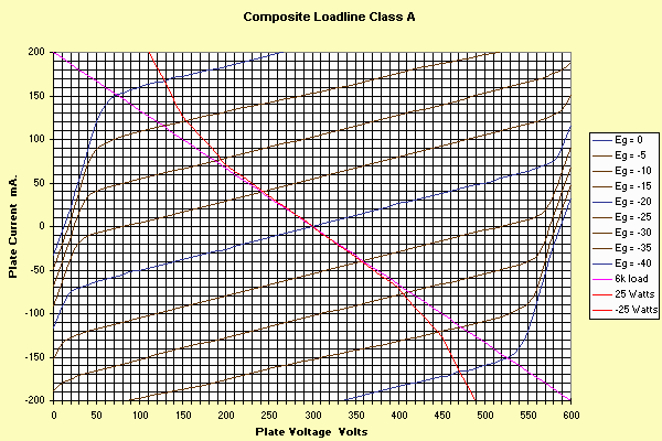
Push Pull Load Line
The same rules we used in the single ended case apply, with one exception: The impedance you plot is the impedance AS SEEN BY A SINGLE TUBE. Thus it is 1/4 the plate to plate load impedance. Lets use a 6000 ohm plate to plate load. In this case, each tube sees 1500 ohm load, and one "point" on the loadline is the 300 volt "0" mA quiescent value. Another convenient point is at "0" volts (namely, 300 volts drop across the 1500 ohm load). By ohms law, this is i = e/r = 300/1500 = 200 mA. As in the SE case, we need to obtain the same 5 currents and 2 voltages to give us the power output and distortion prediction.
Remember the formulas we used:
Po=(Ve-Va)*(Ve-Va)/(8*RL)
HD2=75*(Ia+Ie-(2*Ic))/(Ia+Ib-Id-Ie)
HD3=50*(Ia-(2*Ib)+(2*Id)-Ie)/(Ia+Ib-Id-Ie)
HD4=25*(Ia-(4*Ib)+(6*Ic)-(4*Id)+Ie)/(Ia+Ib-Id-Ie)
These work, with the RL value equal to a single tubes load (1500 ohms in our example).
The values from the graph are: Va=71V, Ve=529V, Ia=151, Ib=77, Ic=0, Id=-77, Ie=-151.
| Power Out | HD2(%) | HD3(%) | HD4(%) |
| 17.5 watts | -0- | 0.7 | -0- |
Notice in the push pull configuration, even order distortion "cancels". Also, of more importance is the fact that the ODD order is reduced over the single ended case, even though the power output is more than double the SE case. Even more important is the significance of the picked load. Again, we picked a loadline that goes through the "knee" of the composite curves. We will show below, that as the bias conditions are altered, the "best fit" impedance changes also, which is quite a change from the triode case.
This is one case where the operation of these two device types is quite different.
The Effect of changing the bias on Pentode Composite Curves
Let's choose a -25 volt bias on the tubes, which will drop the idle current to 60 mA. As I mentioned above, technically, this is still Class A operation. The curves look like this:
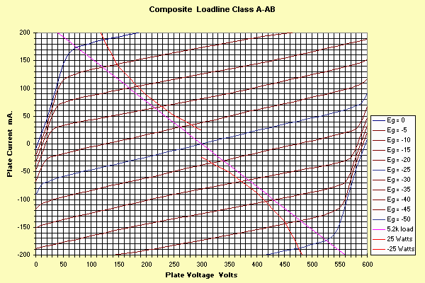
One important item to note is that now, an appropriate load line is 5.2k instead of 6k. (Substantially lower load impedance produces lower power and higher distortion, as does substantially higher load impedance.)
For this condition, The seven values picked from the curve are 74V, 526V, 174, 83, 0, -83 and -174 mA.
| Power Out | HD2(%) | HD3(%) | HD4(%) |
| 19.6 watts | -0- | 1.6 | -0- |
Notice the available power output has increased, but so has the distortion.
This is even more obvious if we move the class of operation into true Class AB:
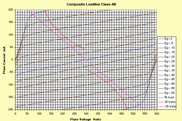
Now, the appropriate loadline has decreased to 5k, but the power output has reached 20 watts.
We can pick 0, -15, -30, -45 and -60 volt points (which gives us full 20 watts output) or choose intermediate points. This is summarized in the following table:
| Power Out | HD2(%) | HD3(%) | HD4(%) |
| 20 watts | -0- | 2.5 | -0- |
| 8.9 watts | -0- | 5 | -0- |
| 1.5 watts | -0- | 3.4 | -0- |
Now you can see the effect of the "compressed" curves around zero bias. The distortion is actually greater at low levels than at maximum output. This is the effect of crossover or notch distortion.
-Steve